Chapter 6
Application of the Atmospheric Model to
Ballooning Part A
Applications of the Atmospheric Model
Modeling applications that come to mind are:
1.The behaviour of weather balloons;
2. Aspects of piloting netted gas balloons such as that used for the Kittinger ascent;
3. Estimating the influence of the atmosphere on Escape Velocity;
4. HARP, High Altitude Research Program, projectiles;
5. The ballistics of a Grenade Launcher.
Cases
The foregoing applications break down into 5 cases each with slightly different
reporting needs. We have called them Cases 0 through 4 as follows:
0 - Expandable Balloons, e.g. Weather Balloons;
1 - Non-Expandable Balloons, e.g. The Kittinger Ascent;
2 - The Kittinger Descent, a special case;
3 - High Altitude Projectiles, e.g. HARP, Escape Velocity;
4 - Ballistics, e.g., Grenade Launcher.
The Parameter Table
The Parameter Table caters to the variety of reporting needs of the cases by providing
some fixed labels, some case dependent labels, and some result dependent labels.
Description of the Object
Our model employs
Lord Rayleigh's approximation for the drag force on a moving
object. In Chapter 2 we arrived at the expression
for the acceleration of such a body due to gravity as:
a
= g - 1/2*1/m*ρ*A*Cd*v2 =
g - k*v2.
We see that there are only three factors in the expression
that are related to the physical characteristics
of the object, i.e., m,
A, and Cd.
The user of the model has the task of distilling
the characteristics of the balloon, falling object, or projectile into values for
these three factors.
The Mass
In Chapter 3 we took buoyancy into account
as a modification to g in the differential equation.
That was because buoyancy creates a force that is opposite to
gravity:
One may think of an effective or buoyant mass mb
for an object with mass m where:
mb = m * (1 - pfluid/pobject)
Under gravity the object will fall if its density is greater than that of the fluid
and rise if less.
The force on the body will be:
Fb = mb* g
The user does not directly input a value for the mass. He does provide an overall density for the object
or system of connected objects and leaves it to the macro to calculate the corresponding
mass from the frontal area A.
The Frontal Area, A
The frontal area A is the cross section of the body in its direction of travel.
We imagine a cylindrical object for which the user provides a radius. It may be thought
of as a sphere that is elongated at its diameter to become a cylinder with ends consisting
of hemispherical caps.
When there are a group of connected
objects such as, in line, a balloon, parachute
and instrument package, one object
such as an inflated balloon, will provide the greatest part of the drag and its area may be chosen. The user specifies the frontal
area by inputting the radius of the hemispherical cap.
The Drag Coefficient
The drag coefficient is shape dependent and can take on a huge range of values,
encompassing
at least three orders of magnitude. See Guns
for an interesting article.
Drag coefficients are obtained by experimental
methods and are frequently kept as industrial and military secrets. We are often left to
guess the
drag coefficient that could apply to any particular case being studied. Roughness of the frontal
area tends to increase drag. Objects can be streamlined to reduce drag.
In some cases we can infer a drag coefficient through consistency checks with various
reported observations. In many cases we are quite relaxed about the precision
of the results and have greater interest in gross behaviour.
Besides, our model neglects all sorts of potential variables such as temperature,
water vapour, rain, snow, wind, up drafts, down drafts, hail and so on.
Connected Objects and Other Considerations
A combination of balloon and payload will have an effective mass that is the sum
of the respective masses. The combination will have a volume that is the sum
of the two volumes and an effective density equal to the ratio of the effective
mass to the total volume. If that effective density is less than that of the surrounding atmosphere, the balloon and its payload will rise.
For ballooning, the important factor is the effective density that is achieved and
its relationship to the density of the surrounding
atmosphere.
For projectiles, a long thin object will generally be assigned a higher density in accordance
with its length.
Slender projectiles moving in air tend to tumble and have an erratic
trajectory. For this reason they are either spun at launch by a rifled barrel or
employ tail fins.
Weather Balloons
A weather balloon is made from a highly flexible material, often Latex. It is inflated
with a light gas such as hydrogen or helium and carries a radiosonde and, sometimes,
a parachute.
Similar devices are employed by amateur groups in hobby ballooning.
Weather balloons may attain altitudes of ~ 40,000 metres before they burst from
over expansion.
The Expandable Balloon case requires a special user input, the Balloon Expansion
Factor. This factor is used by the macro to adjust the density of balloon
and payload as atmospheric density changes during the flight. The radius of an expandable
balloon is increased by the macro as less dense atmosphere is encountered and vice
versa. The limit provided by the factor is a restriction on radius. A factor greater
than 0.0 restricts the radius change to that multiple. The factor 0.0 indicates
that an object may neither expand nor contract.
In Case 0, the Weather Balloon, the balloon disintegrates when it reaches the expansion
limit. In Case 1, the balloon simply expands no further when the limit is
reached.
See Weather Balloon for other details.
A Weather Balloon Example
The Web-based 2D Calculator version of the spreadsheet
is used for the examples in this topic. That calculator is available at the
end of this chapter and from the upper row of navigation tabs.
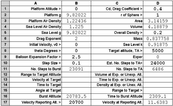
The parameter table follows:

The Inputs
The user is interested in a launch from sea level and puts a 0 in cell B1. The macro
then provides the values for B2 through B6. The value in B6 is a reminder that we
are presuming that drag force is proportional to the square of velocity.
The user puts the value of 0 in B7 and B8 as the balloon is not being given an initial
push at launch. It is simply being released.
The user puts the limit by which the balloon's radius may expand before bursting
in B9. This is a value that is generally provided by the balloon's manufacturer.
The user puts the desired step size for the calculation in cell B10. It may
be borne in mind that the first step will always consist of 10 graded smaller steps
that have the purpose of, improving computation when initial values are subject
to rapid change as can occur when a projectile decelerates in atmosphere.
The user provides the value 0.4 in D1. This value would be consistent with a rough-surfaced
spherical shape for the balloon. Perhaps 0.4 will also take into account the drag of the attached parachute and instrument case.
The balloon as inflated at sea level has a radius of one metre. The value 1 is placed
in D2. (Weather balloons can be obtained in a variety of sizes as needed for different
payload masses.)
The macro provides values for D3 and D4.
The user provides a density value for the system that is smaller than that
of the atmosphere at sea level. The smaller the difference the slower will
be the ascent.
The macro then provides values for D6 and D7.
D7 gives the sea level value of the k value that appears in Lord Rayleigh's
approximation for the drag force on a moving object:
a = g - k*v2.
Our k is not a constant but is a variable that is dependent on altitude.
A value for D8 can be more useful in other cases but a value placed here for Target
Altitude will cause the macro to report the number of calculation steps taken
to just exceed that altitude at D11.
The user puts a 0 in cell D9 to indicate to the macro that the data applies to
the Weather Balloon case.
The value the user places in D10 constrains the total number of steps that will
be calculated by the macro. The macro will stop computation at that number of steps
even though an objective may not have been reached.
There may be cases for which the velocity reached at a selected altitude is of interest.
A user altitude value placed in B17 will cause the macro to report the associated
velocity in cell D17.
Macro operation has two phases. In the first phase the macro provides cell
values in the parameter table in accord with user inputs and any changes made thereto, thus acting as a handy calculator.
In the second phase the macro calculates all the required steps and produces a step-by-step
table in which intermediate values can be seen and from which
graphs are constructed.
Examples of the possible application of the handy calculator can be as simple as calculating
sphere properties such as cross section area volume or mass, to providing
a value for g at
a given altitude or the value for atmosphere density at a given altitude.
The Outputs
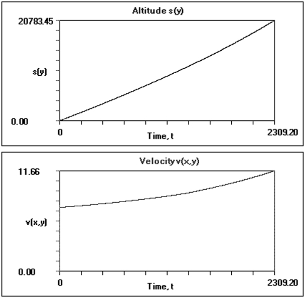
In this case the balloon bursts after 23,091 steps
at an altitude of 20,783.5 metres at ~ 38.5 minutes after launch.
Its upward velocity at the 20,700 metre level was
~11.64 metres per second.
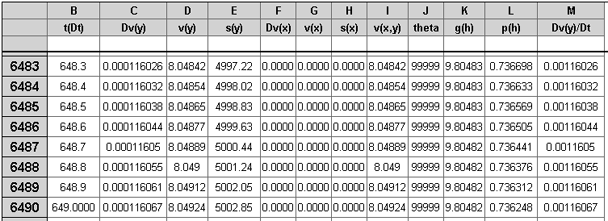
It reached a Target Altitude of 5,000 in 6486 steps. At 0.1 second per step, that's
at nearly 11 minutes after launch. From these values we deduce an average ascent
rate to the 5,000 metre level as 7.71 metres per second, less than that seen
at the 20,700 metre level.
A portion of the table that is output showing the 5,000 metre level follows:

The altitude and velocity graphs are seen next:

Had the balloon a greater expansion factor it would have
reached a higher altitude before bursting.
Had the overall density been greater, e.g. more payload, the balloon would have
risen at a slower rate.
Next
The next topic explores characteristics of pressurized
balloons as a further example
of the application of the entire atmosphere model.