Chapter 9
Navigation of Orbiter from MECO to the ISS - Maneuvering in Orbit - Solver Revisited
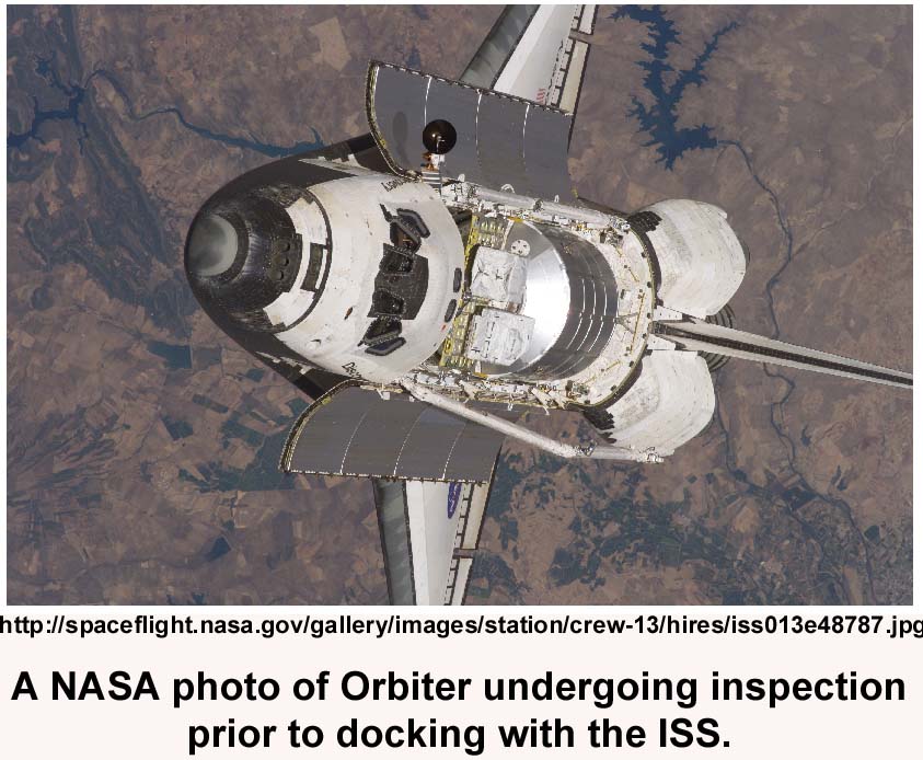
The image below shows Orbiter at an altitude of about 300 km above the Earth in
the ISS orbit just prior to docking with the space station.
Adaptive Conditional Feedback Control Navigation Process
In this topic we further describe elements of an Adaptive Conditional Feedback Control Navigation
Process and illustrate it using our spreadsheet. A 1955 paper "Conditional
Feedback Systems -----" is available from the Download tab.
Describing the Navigation System
Navigation of Orbiter
in Earth Orbit bears no resemblance to the experience of driving a car. In orbit
he influence
of gravity on motion is not constrained by the surface of a roadway.
It is easy to steer from your own location to that
of your destination when there
are wheels on the ground.
The main rocket engines
provide a nearly fixed amount of thrust when on and none when off. Orbiter does not quickly decelerate when the engines are off.
It continues with little atmospheric or other friction to slow it.
On Earth cars may travel at different speeds along the same roadway. All objects
in a given Earth orbit travel at the same speed. Changing the speed changes
the orbit.
The difficulties of navigation in orbit suggest that computers be employed in the
navigation process, as will now be described.
The navigation process consists of Objectives and the Commands that are designed
to achieve those objectives.
A purpose of the 'Model Computer' is to design the Commands. It does this
by sequentially adjusting command values
on a model of the vehicle and its environment
until they are seen to be what is needed to achieve the objectives.
An Example of Command Design
As a simple example, presume that the vehicle is coasting in a low and very
circular Earth orbit. Apogee and perigee are equal at an altitude of 300 km.
Then
suppose, as an objective, that it is desired to raise the altitude of the vehicle's
apogee by 200 metres while maintaining the current 300 km perigee altitude.
Adding thrust to change the vehicle's velocity should accomplish this but how
much thrust in what heading?
Suppose further that we require the thrust to take place over a 175 second interval
as we are approaching the use of another objective and want the changes to occur quite
slowly so that corrections can be readily made if required.
The objectives are provided to the Model Computer, which by fast iteration, akin
to trial and error, determines
the command to be given to the Course Computer.
The Model Computer is constantly aware of the vehicle's state via its connection
to the State Computer and within seconds the command "Apply a force
of 30.857 Newtons for a period of 175 seconds at the current azimuth angle and with
0.0 degrees of elevation." is presented to the Control Computer.
That is not the end of it. The Model Computer had created a detailed path that the vehicle should follow after it has been given the command. However, there are many influences that may cause the actual path taken
by the vehicle as provided by the State Computer, and the path predicted by the model, to differ as time passes.
Any significant departure from the objective requires alteration of the Course Computer's
current commands or the issue of corrective commands. For example, reduce the
time of the thrust by a certain amount or decrease the elevation angle of the thrust
by an amount. Additionally it may be found necessary to update the model. This is an adaptive conditional feedback process.
Importantly, the forgoing section has introduced
the notion of the error between the result expected from the command and the result
realized by the command being used to correctively alter the command, and possibly
the model, in a manner that will reduce the error. This is the essence of
our navigation system.
This simple example is a case of delicate manoeuvring
with the RCS. The OMS engines operate with
a very much greater combined fixed thrust of ~53,400 Newtons and are not useful
for delicate positioning.
The Course Computer
There are two OMS engines. The Course Computer must do the detailed work of controlling,
instant by instant, the angles of each thrust gimbal with respect
to the orientation of the vehicle and the vectoring of the RCS thrust when it comes
into play.
The bearing command that it receives is a bearing that is relative to the tangent plane
at every position along its path during the interval that the corresponding thrust
is applied. It employs the planned course that accompanied the Thrust and Bearing
command, passed to it by the Model Computer, to compute the time-varying
angles required along the path for the gimbaled thrusters in order to maintain
the required bearing relative to the current tangent plane.
Spreadsheet Model used to find Course Commands
The fast iteration method of finding course commands is illustrated using the spreadsheet.
Specialized Solvers are added to the
combination of Input Table and the spreadsheet model described in Topic 3 of Chapter
7.
The Nature of a Solver Revisited
The ingredients of a Solver are Objectives, calculated
Results from a model, an Error, Sensitivities and Controllables.
The model produces Results. Results are compared with
Objectives to produce an Error. Numerical differentiation provides the sensitivity
of the error to each controllable. The sensitivities provide a vector of changes
to be made to the controllables that reduce the error.
The process is iterative and reduces the error with each iteration so that the
Results become closely equal to the Objectives.
In our application the controllables are the elements of a Course Command.
Initial values of the controllables are applied to the model and the result is a
computed path taken by the vehicle.
Data from the computed path is compared with data from the objective to compute an error.
The sensitivity of the error to small changes in each of the controllables is determined
for each controllable by recomputing the error when a small change is made to that
controllable.
Each controllable is then modified a small amount in proportion to its sensitivity
and will thereby reduce the total error a small amount.
This process repeats, iterates, until the course command results in a computed path
that is adequately close to the objective path.
The Combination - the Model Computer
The addition of the Input Table and Solver to the three-dimensional spreadsheet
model of rotating earth and atmosphere created a powerful tool capable
of solving for thrust vectors that will take a space vehicle from one state to another.
The method could have been employed at lift-off to guide the main engines
and booster rockets, to reach a desired altitude and desired inclination at the time
that the boosters are dropped. It could be used thereafter to guide the main engines
to maximum altitude
and velocity at the point called MECO where
the near empty External Fuel Tank is jettisoned.
Example - Correcting the Model of Orbiter's OMS Engines
Suppose that the parameters that were used to represent the MECO state of Orbiter,
prior to the first burn, were highly
accurate position, velocity and orientation
data,
provided by the State Computer.
The OMS engines have not been
previously operated and we are unsure of their precise thrusts and their balance.
Orbiter's on-board Model Computer is able to use the known MECO state
to compute the thrusting times and angles based on the nominal thrust of the OMS
engines and their nominal response to bearing commands to reach a desired position
in the ISS orbit.
On any particular mission the thrusts of the two OMS engines
may each differ from their nominal values. Imbalance in the thrusts
will cause some offset to occur between a commanded thrust and bearing and the resulting
achieved thrust and bearing.
If the OMS engines and bearing controls were at nominal, all would be well and Orbiter
would reach its objective. If not, how could corrections for thrusts, burn
times and bearings be obtained?
Finding the Corrections
The object is to find out,
early in the first OMS burn, how much the actual OMS
engine thrust differs from its nominal value and by how much Orbiter's response to a bearing
command differs from that desired.
The procedure
to determine such an imbalance can be demonstrated by supposing that the thrust and
azimuth values of the first burn did not produce the trajectory that
was calculated for the first burn.
We show the first 10 seconds of the altitude of that calculated trajectory next:
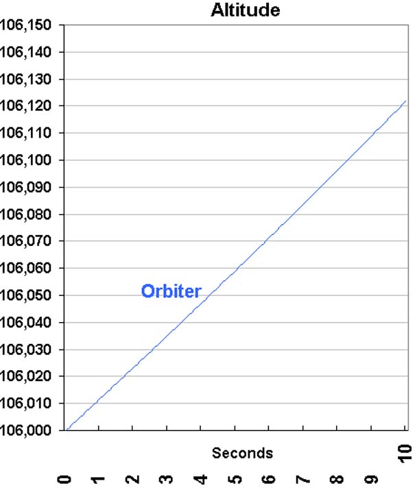
Fundamental state data is produced by the Model Computer every 0.01 seconds. These
are the x, y, z position values and the corresponding Vx, Vy, Vz velocity values.
All other values such as latitude, longitude, bearing angles, altitude, speed and
acceleration are derived from the fundamental state data.
Orbiter's State Description and Applied Thrust
at a Bearing
When thrust at a bearing is applied for a time to Orbiter, the state description
of Orbiter will change smoothly from one state to the next.
Given a sequence of states that occur, is it possible to determine the causative
thrust and bearing?
The answer is, as Newton put it, "pretty nearly".
The x, y, z states expected of Orbiter after each of the first 10 seconds of burn from MECO
with a thrust of 53,400 Newtons at an Azimuth of 95.327 degrees are shown next:
Now suppose that actual position, velocity, and heading of Orbiter, were
available at one second intervals from the State Computer and represented in
x, y, z format as shown next:
(These demonstration values were obtained by presuming a thrust of 52,400
Newtons and an Azimuth of 97.327
degrees.)
Solver, the atmospheric model and the Input Table were the given the objective of
matching the first five rows of this table. The result is shown next:
In the first 5 seconds after MECO an actual value of 52,400
Newtons has
been found for the thrust of the particular OMS engines, as has a 2.0-degree
offset
from nominal of the Azimuth controller.
The x, y, z state of Orbiter 5 seconds after MECO, may now be used to compute corrective new burn times and adjusted azimuth values, for the first and second
burns that are required to achieve the orbit of the ISS.
As there are 9 seconds remaining of the first burn there is time in which its azimuth
and its thrusting time can be corrected to bring the path closer to a desired path.
In our system of navigation, navigation corrections like those that have been described for the
first few seconds after MECO, are part of a continuous course correction
process that takes place from launch up to the point of close proximity to the space station.
Comparison of the calculated position states with actual position states can be
used to refine thrust values, the elevation angle and bearing of thrusts and to refine the mass and
rate of loss of mass values of the Orbiter model.
Over a longer-term basis, buoyancy, lift values, and
even Cd and effective area could be refined so as to improve the model as the trajectory
continues.
Parameters that have
the least effect on the trajectory require
greater observation time for their determination than those parameters that that
have larger effect.
It is also quite possible that each mission of Orbiter could
be used to contribute some to the atmospheric parameters of the Orbiter model.
Using the Spreadsheet - Maneuvers in Orbit
Circular Orbits
An object in ideal circular orbit in vacuum has a constant
altitude and a constant tangential velocity. This is nearly true of an object
in orbit at 300 km above the Earth. Such an orbit is very sensitive to velocity.
The effect of 0.1 metre per second changes in an orbital speed of ~7730 m/s is seen next:
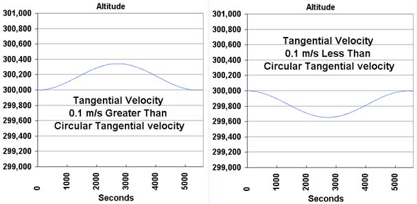
An increase in velocity resulted in an eccentric orbit
with perigee at 300km. A decrease resulted in an eccentric orbit with apogee at
300km.
Neither an Input Table nor a Solver
is required to create this example.
Velocity and Energy
The velocity needed to maintain a near-circular orbit over a range of altitudes and with,
for interest, the total, kinetic and potential energy of an Orbiter in
those orbits,
is shown next:
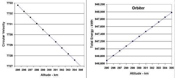
The orbital energy must be shed to the atmosphere on a return flight to Earth. For
perspective, a Canadian electrically heated and cooled single-family dwelling might
use 15,000 kWh of electrical energy per year.
Increasing the Altitude of an Orbit using a Vertical
Burn with the RCS
Consider Orbiter in a circular orbit at 300 km. There is a need to increase
the altitude by one km. One might imagine that a short vertical burn with the RCS
would be helpful.
See the effect of such a burn in the left panel of the image that follows.

After a waiting time to reach the 301 km apogee, the orbit is circularized at that
altitude, right panel. In total, about 300,000 Newton seconds was employed.
It took about 1,380 seconds to increase the altitude of the orbit by 1 km.
The azimuth of the circularizing burn was chosen to maintain an inclination of
51.6 degrees.
The RCS might possibly, instead, have been used to rotate Orbiter to allow the OMS engines
to thrust vertically and later tangentially. If so, at nominal OMS thrust, a burn time of
about 2.27 seconds would have been required to reach the 301 km altitude
and about 3.35
seconds would have been required to circularize. The OMS engines can be operated
for as short two seconds but it seems unlikely that they would be considered precise
enough for this application.
Increasing the Altitude of an Orbit using Tangential
Burns with the RCS
The difference in this case is that a rise in altitude of one km requires 25% of
the force needed for the vertical burn if a tangential burn is employed.
See the left panel in the image next:
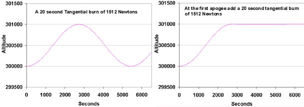
Note that apogee in this case is delayed by factor of two as compared with the use
of vertical force.
Note
also that the circularizing force has the same value as that employed to reach
the 301 km altitude with the vertical burn, as might be expected.
Also, given the large inertia of Orbiter, there is not much difference in the effect
provided by a 20 second application of 1512 Newtons and the effect of a 30,240
Newton Second impulse. For this reason, the forces employed could be increased
and applied for proportionately less time, or decreased by some amount and applied
for more time, and have much the same effect.
In raising the altitude of an orbit it appears that tangential thrusting requires
less Newton Seconds than does vertical thrusting but more time is required
to
reach the new orbit.
Choosing a thrust elevation that is intermediate between 0 and 90 degrees provides
flexibility in the time taken to reach the higher orbit.
When maneuvering near rendezvous, vertical thrusting may become quite important.
Next
A first pass rendezvous of Orbiter and the ISS. A delayed rendezvous. Summing up.